Predicting Drug Combinations
Introduction
Drug combinations can be remarkably effective medicines. For example, antiretroviral
therapy (ART) has dramatically reduced the HIV-related mortality rate. On their own,
the constituent drugs of ART are ineffective - HIV rapidly mutates and acquires
resistance to them. When the constituent drugs of ART are combined, any HIV particles that acquire resistance to a single drug are eliminated by the others. Presumably, multi-drug cancer therapies will also be more effective than single drugs.
One approach to finding a candidate drug or drug combination is through Connectivity Mapping. This approach measures how gene expression is changed in response to a disease and then searches for drugs that cause the opposite changes in gene expression. Drugs found in this manner are predicted to reverse the gene expression changes caused by the disease and thereby reverse the disease. This approach was taken up by the Broad Institute, when they assayed how gene expression is changed in response to 1309 different drugs.
This may seem like a large number of drugs in which to find candidates. However, if you also include all unique two-drug combinations of the 1309 assayed drugs - this represents a staggering 856086 potential medicines. It is currently unfeasible to assay all these combinations, but their expression profiles can be predicted.
In this post, I show you the approach that I took to predict drug combinations for my Bioconductor package ccmap. I first implement a neural network in Python followed by a gradient boosted random forest in R. Along the way, I introduce the concepts of data augmentation and stacking. You can follow along by downloading the training data from here.
Training Data
The training data consists of all microarray data that I could find from GEO where single treatments and their combinations were assayed. In total, 148 studies with 257 treatment combinations were obtained. For all the studies used, only 3483 genes were common to all. As such, a separate neural network was trained to infer any missing values (not covered here). Let’s load up the data:
import numpy as np
from sklearn.utils import shuffle

# Assuming the training data is in your working directory:
X = np.load('X.npy')
y = np.load('y.npy')

X.shape  # 257 samples x 11525 expression values for each of two treatments
y.shape  # 257 samples x 11525 expression values for combination treatment

# shuffle data
ids = shuffle(range(y.shape[0]), random_state=0)
X   = X[ids]
y   = y[ids]
A Tale of Two Models
Let me tell you the story of Simple Model and Hopeless Model.
Simple Model, like her name suggests, takes a simple approach to predicting how gene expression will change in response to a combination of two treatments. Simple Model looks at each gene one at a time and asks: “What was the effect of the two individual treatments on this gene?”. Simple model then does something reasonable, but simple, like averaging the effect of the two individual treatments.
from __future__ import division

# fraction of correctly identified up and down regulated genes
def accuracy(y, yhat):
    num_equal = np.sum(np.sign(y) == np.sign(yhat))
    num_total = y.shape[0] * y.shape[1]
    return(num_equal / num_total)

# accuracy of Simple Model (78.96%)
avg = (X[:, :11525] + X[:, 11525:]) / 2
accuracy(y, avg)
Hopeless Model is much more ambitious and thinks Simple Model a bit simple. In order to predict how gene expression will change in response to a combination of two treatments, Hopeless Model looks at how the first treatment affected all 11525 genes AND how the second treatment affected all 11525 genes. By doing this, Hopeless Model thinks he can find some relationships that simple model has no chance of discovering. Unfortunately, Hopeless Model only has 257 samples and so a lot of the relationships he finds only work well on these samples. They don’t apply very well to data that he hasn’t observed (See here for a description of prerequisites and the various neural network parameters):
from lasagne import layers
from nolearn.lasagne import NeuralNet, TrainSplit
from lasagne.updates import nesterov_momentum
from lasagne.nonlinearities import very_leaky_rectify
import theano

# For Adaptive Learning Rate/Momentum ----

def float32(k):
    return np.cast['float32'](k)

class AdjustVariable(object):
    def __init__(self, name, start=0.03, stop=0.001):
        self.name = name
        self.start, self.stop = start, stop
        self.ls = None

    def __call__(self, nn, train_history):
        if self.ls is None:
            self.ls = np.linspace(self.start, self.stop, nn.max_epochs)
        epoch = train_history[-1]['epoch']
        new_value = float32(self.ls[epoch - 1])
        getattr(nn, self.name).set_value(new_value)


# Hopeless Model ----

net = NeuralNet(
    layers=[
        ('input',   layers.InputLayer),
        ('dropout1', layers.DropoutLayer),
        ('hidden',  layers.DenseLayer),
        ('dropout2', layers.DropoutLayer),
        ('output',  layers.DenseLayer),
        ],
    # layer parameters:
    input_shape          = (None, X.shape[1]),
    dropout1_p           = 0.85,
    dropout2_p           = 0.5,
    hidden_num_units     = 2500,
    hidden_nonlinearity  = very_leaky_rectify,
    output_nonlinearity  = None,
    output_num_units     = y.shape[1],

    # optimization method:
    train_split          = TrainSplit(eval_size=0.2),
    update               = nesterov_momentum,
    update_learning_rate = theano.shared(float32(0.01)),
    update_momentum      = theano.shared(float32(0.9)),
    regression           = True,
    max_epochs           = 5000,
    verbose              = 1,
    on_epoch_finished    = [AdjustVariable('update_learning_rate',
                                           start=0.01, stop=0.00001),
                            AdjustVariable('update_momentum',
                                           start=0.9, stop=0.999)],
    custom_scores        = [("acc", lambda y, yhat: accuracy(y, yhat))]
    )

np.random.seed(0)
net.fit(X, y)

# accuracy of Hopeless Model (66.95%)
Data Augmentation
Hopeless Model, realizing his folly, figures out a clever way to improve his predictions. He reasons that the expression of each gene is affected by two separate treatments (by amounts dA and dB), and that the effect of the combined treatment should be similar irrespective of which treatment is responsible for which effect. This reasoning allows him to randomly swap dA and dB for each gene and thereby gives him access to an essentially limitless amount of training data (lines that end with #! indicate a change from the previous model):
from nolearn.lasagne import BatchIterator
from random import choice, sample

# Class to Swap dAs and dBs ----

class FlipBatchIterator(BatchIterator):

    def transform(self, Xb, yb):
        Xb, yb = super(FlipBatchIterator, self).transform(Xb, yb)

        # number of samples and genes
        ns = Xb.shape[0]
        ng = Xb.shape[1] // 2

        # for random half of genes and samples, swap dA and dB
        sw = [choice([0,1]) for _ in range(ng)]

        dA = [ i    +(s*ng) for i, s in zip(range(ng), sw)]
        dB = [(i+ng)-(s*ng) for i, s in zip(range(ng), sw)]

        cols  = dA + dB
        rows  = sample(range(ns), ns // 2)

        ind_orig = np.ix_(rows, range(ng*2))
        ind_flip = np.ix_(rows, cols)

        Xb[ind_orig] = Xb[ind_flip]

        return Xb, yb


# Augmented Hopeless Model ----

net = NeuralNet(
    ...
    # optimization method:
    batch_iterator_train = FlipBatchIterator(batch_size=70), #!
    ...
    )

np.random.seed(0)
net.fit(X, y)

# accuracy of Hopeless Model (up from 66.95% to 68.21%)
Stacking
Hopeless Model is feeling a bit down about his accuracy and seeks consolation from Simple Model. While consoling her friend, Simple Model realizes that there are certain situations when she can make a better prediction by considering both Hopeless Model’s predictions AND the effect of the two individual treatments on a given gene. This news sure cheers up Hopeless Model!
This is a description of the machine learning approach called stacking (MLwave has a fantastic guide to stacking and other variations of model ensembling). One important subtlety of stacking is that in order for Simple Model to effectively learn when Hopeless Model’s predictions should be incorporated, Hopeless Model can’t have been trained on the data that he is providing predictions for. If he has, Hopeless Model’s predictions will seem strangely accurate and end up being weighted too heavily.
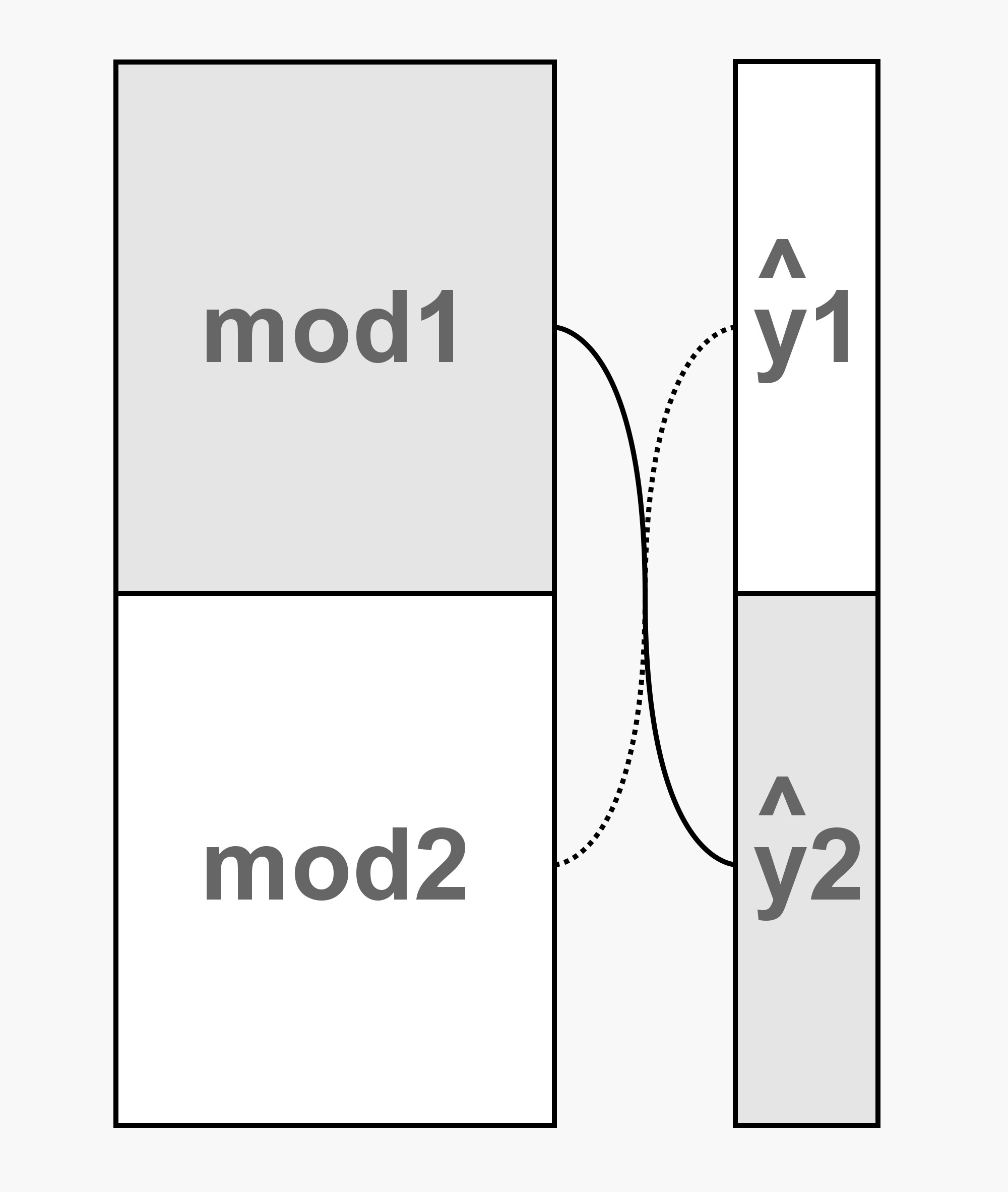
To get around this, we train two separate Hopeless Models. Each sees half of the data and then provides their predictions for the other half (figure below). By doing this, we get Hopeless Model’s predictions for the entirety of the training data and ensure that those predictions are good reflections of Hopeless Model’s ability.
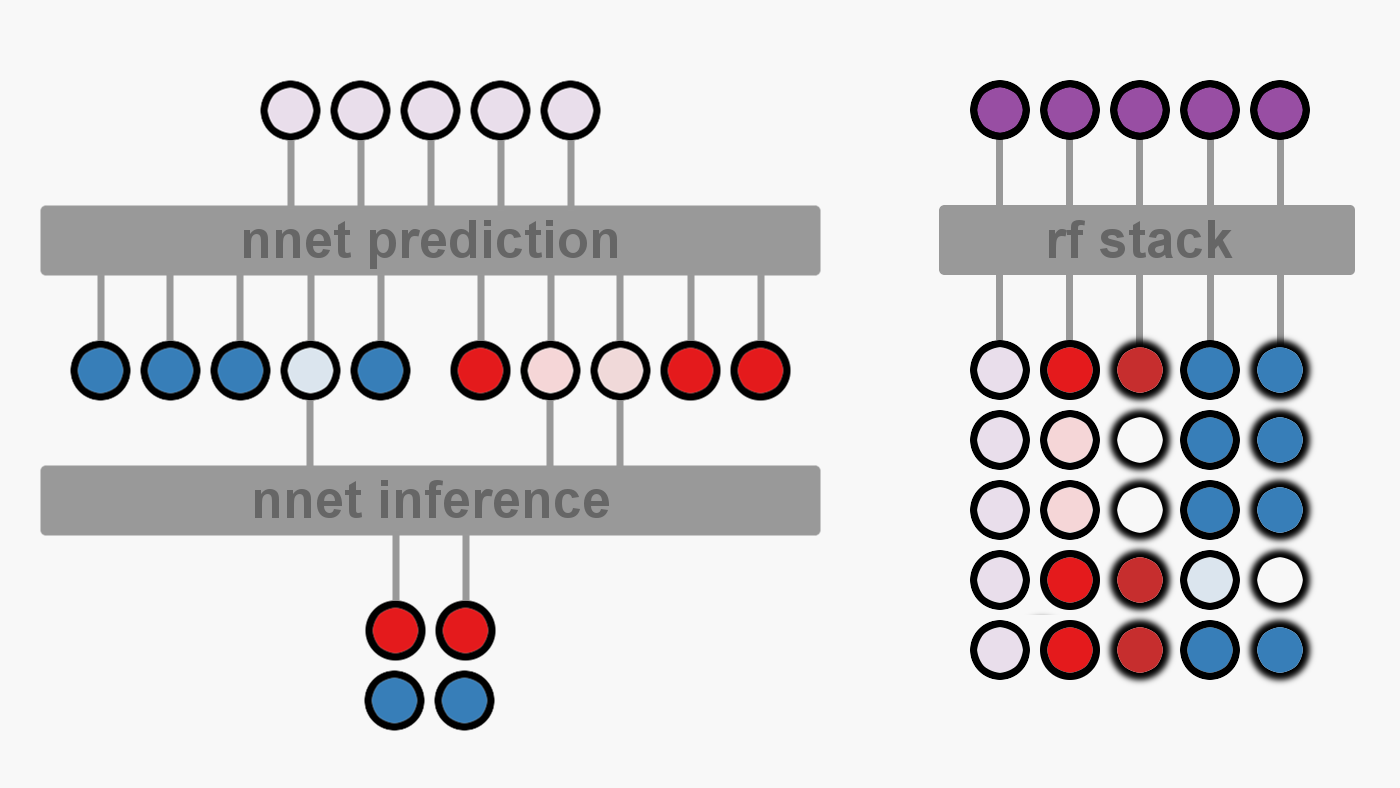
For our purposes, Hopeless Model’s predictions will be stacked with a gradient boosted random forest. Hopeless model will make his predictions (figure below on left - transparent purple circles) and then pass them to the random forest (figure below on right). Each sample provided to the random forest will contain the information for only a single gene from one study. For each sample, the random forest will have access to Hopeless Model’s prediction and to the effect of the two individual treatments (both effect sizes - solid red and blue circles, and variances - feathered red and blue circles). Note that xgboost doesn’t mind missing data so we don’t need to infer the missing variances.
Let’s remove the evaluation set and train our two Hopeless Models, each on half of the data:
# divide data in two
X1 = X[:128]
X2 = X[128:]

y1 = y[:128]
y2 = y[128:]


# Hopeless Model 1 ----

net1 = NeuralNet(
    ...
    # optimization method:
    train_split = TrainSplit(eval_size=0.0), #!
    ...
    )

np.random.seed(0)
net1.fit(X1, y1)

# predict y2 from X2 using net1
y2_preds = net1.predict(X2)


# Hopeless Model 2 ----

net2 = NeuralNet(
    ...
    )

np.random.seed(0)
net2.fit(X2, y2)

# predict y1 from X1 using net2
y1_preds = net2.predict(X1)
Before training the random forest stacker, we first need to reshape the training data and Hopeless Model’s predictions. We will also reapply the same shuffling and reshaping to our variances and add them to the training data for our stacker:
# load and shuffle variances
Xv = np.load('Xv.npy')[ids]

# stack preds for each sample (rows) on top of each other
preds = reshape(np.vstack((y1_preds, y2_preds)), -1, 'A')

# stack samples on top of each other with dA and dB for each gene side by side
X  = np.transpose(np.vstack((reshape(X[:,:11525],  -1, 'A'),
                             reshape(X[:,11525:],  -1, 'A'))))
Xv = np.transpose(np.vstack((reshape(Xv[:,:11525], -1, 'A'),
                             reshape(Xv[:,11525:], -1, 'A'))))
y  = np.reshape(y,  -1, 'A')

# concatenate preds, X, Xv, and y
train = np.c_[preds, X, Xv, y]

# save result for xgboost training
np.savetxt("train.csv", train, delimiter=",")
Pirates Love R
What is a pirates favorite programming language? Rrrrrrrrr!
One of the few things I prefer Python for is its neural network modules. As such, I am going to perform the stacking in R. Also, the final model is implemented in R (as part of the ccmap package) so I had to transfer over the trained neural networks from Python to R. Thankfully this is relatively straightforward. To do this for net1, first extract and save the weights in Python:
import pandas as pd

# net1 weights and biases
W1 = net1.get_all_params_values()['hidden'][0]
W2 = net1.get_all_params_values()['output'][0]

b1 = net1.get_all_params_values()['hidden'][1]
b2 = net1.get_all_params_values()['output'][1]

# save them as csv
pd.DataFrame(W1).to_csv("W1.csv", header=False, index=False)
pd.DataFrame(W2).to_csv("W2.csv", header=False, index=False)
pd.DataFrame(b1).to_csv("b1.csv", header=False, index=False)
pd.DataFrame(b2).to_csv("b2.csv", header=False, index=False)
Then load the parameters in R:
library(data.table)

W1 <- as.matrix(fread("W1.csv"))
W2 <- as.matrix(fread("W2.csv"))

b1 <- fread("b1.csv")[, V1]
b2 <- fread("b2.csv")[, V1]
Our Hopeless Model’s prediction function is relatively straightforward as well:
predict.net <- function(W1, W2, b1, b2, X) {
    # add bias to dot product of input and W1 matrices
    z2 <- X %*% W1 + b1

    # hidden non-linearity is very leaky rectifier
    a2 <- pmax(z2/3, z2)

    # add bias to dot product of a2 and W2 matrices
    # output non-linearity is none
    return (a2 %*% W2 + b2)
}
And our final stacker is trained as follows:
library(xgboost)
library(data.table)

# load data to train stacker on
train <- fread("train.csv")
names(train) <- c("net_preds","drug1_dprime", "drug2_dprime",
                  "drug1_vardprime", "drug2_vardprime", "combo_dprime")

# seperate into X and y
X <- train[, !"combo_dprime", with=FALSE]
y <- train$combo_dprime

# evaluation metric
accuracy <- function(preds, dtrain) {
    labels <- getinfo(dtrain, "label")
    acc <- sum(sign(preds) == sign(labels)) / length(labels)
    return(list(metric = "acc", value = acc))
}

# build a xgb.DMatrix object
dtrain <- xgb.DMatrix(data=as.matrix(X), label=y, missing = NA)

# for adaptive learning rate
my_etas <- list(eta = c(0.5, 0.5, rep(0.15, 6)))

# cross validation
history <- xgb.cv(data = dtrain, nround = 8, objective = "reg:linear",
                  eta = 0.5, max.depth = 15, nfold = 5, prediction = TRUE,
                  feval = accuracy, callbacks = my_etas)

# final stacker
xgb_mod <- xgboost(data=dtrain, nround=8, objective = "reg:linear",
                   eta=0.5, max.depth=15, callbacks = my_etas)


# Model | Accuracy | Incorrect
#       | (%)      |(per 11525 genes)
# ----- | -------- | ------------
# avg   |  78.96   | 2424
# +vars |  79.13   | 2405 ( -19)
# +nets |  79.72   | 2338 ( -86)
# +both |  80.17   | 2284 (-140)
Evaluation
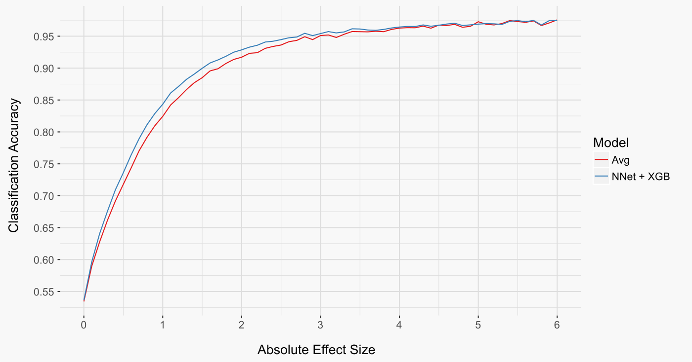
One informative way to analyse our models is to look at how well they do as a function of the absolute effect size of the combination treatment (figure below). Both models make almost perfect predictions at high absolute effect sizes. In contrast, both models struggle to decide if a gene is up or down regulated at small absolute effect sizes. These trends make sense: the smaller the effect size, the more likely it was due to chance and will not be reproducibly positive or negative. Perhaps unsurprisingly, it’s only for intermediate effect sizes that the stacker model has the advantage. These cases are neither trivial to predict, such as those with large absolute effect sizes, nor virtually impossible to predict, such as those cases with effect sizes very close to zero.
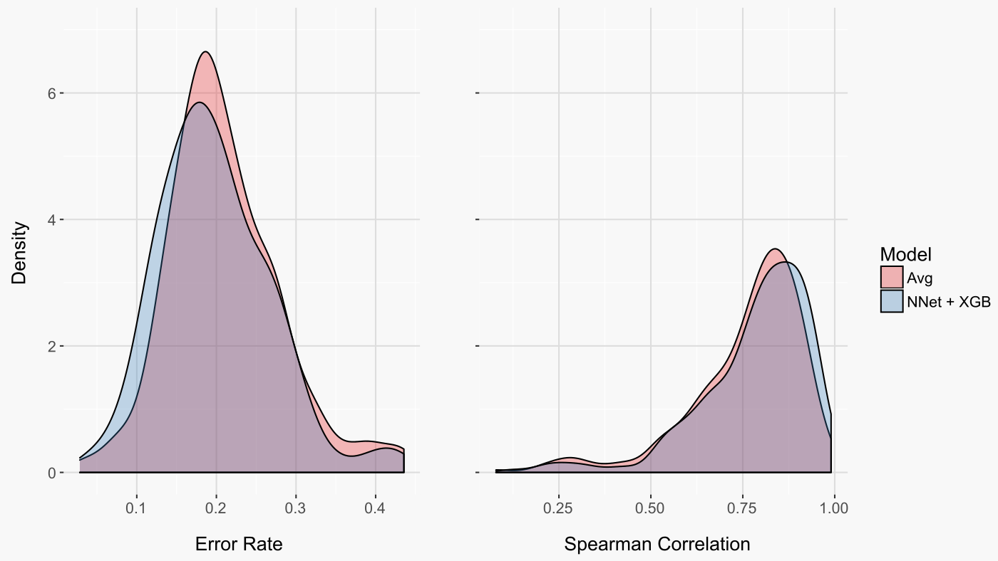
Another informative way to evaluate our models is to look at the distribution of error rates across the 259 treatment combinations (figure below on left). Interestingly, this perspective reveals that a small number of treatment combinations were either almost perfectly predicted (very low error rate) or predicted seemingly at random (error rate near 50%).
In addition to considering the accuracy of classifying a gene as down- or up-regulated, it is also relevant to consider if genes were accurately ordered from the most down-regulated to the most up-regulated. The correlation between ranks, or spearman correlation, provides just this measure. Again, both models did quite well, with a slight advantage to the machine learning model (figure below on right).
Summary
In this post I trained a model to predict gene expression changes in response to a drug combination based on the measured gene expression changes after treatment with the individual drugs. As compared to a model that simply averages the effects of the two individual treatments, the final model is more accurate at both classifying genes as up- or down- regulated and at ordering genes from the most down-regulated to the most up-regulated. To build this model, I employed the machine learning techniques of data augmentation and stacking. I may have also told a really bad fairy tale and made an awesome programming joke about pirates.